Manipulating CSV Data Files in Excel

The comma-separated-value file that you just received can be easily manipulated in Microsoft Excel to produce lists and reports of the data you asked for. If you are using Outlook for Windows, double-click on the attached CSV file and choose Open it to see your data in Excel. Other email clients may need to save the file to your hard disk first.

If you are using a Macintosh, your computer may not automatically load the CSV into Excel. After saving the file to your desktop, ctrl + left click (two-button mouse), select Open With, and choose Microsoft Excel. (If Excel is not listed as a choice, select Other and then show All Applications.) You may wish to change your default settings so that MS Excel will be the default application for all CSV files. If so, follow the following steps:

1. Save file to desktop

2. Click once to select the file

3. Option (or Apple key) + I to Get Info

4. Open with section: Click in drop down box

5. Select MS Excel (you may need to scroll)

6. Click Change All button

7. Choose MS Excel

Working with the spreadsheet

In order to more easily view and manipulate the data, I suggest you begin with the following two steps:

1. Choose Data; Filter; Autofilter. This will turn on the column filters, making it easy for you to select particular groups of data.

2. Click on the small box in the upper left corner of the spreadsheet to select the entire sheet. Then point at the small vertical line between the A and B column headings. When the mouse pointer changes to show a two-headed arrow, double-click to size all of the columns in the spreadsheet at once.

To select a particular set of records, you can now click on the drop-down menu on a column heading and select a value. If there are students that you don’t wish to include in your report, you may right-click on any of their data fields and Delete the Entire row.

To sort the data, click on any cell in the column you want to sort by and then click either the A-Z or the Z-A button on the Formatting toolbar. You may also choose Data/Sort on the menu bar for more complicated sorts.

If you plan to print a list, there will probably be data fields that you don’t wish to include. You can right-click on any column letter and select Hide. Use Print Preview to see how your report will look on the page and change column widths as necessary.

You may want to format some numeric data columns, such as the ID, that are imported in Excel as numbers without leading zeros. To change the way these columns look, click on the column letter, choose Format/Cells…, select the Custom Category, and enter a format in the Type blank with leading zeros, such as 000000000 or 000-00-0000 or 0000-0000. The undeclared major code, 0000, has been converted to UNDE to avoid the need for this step when displaying major codes.

If a field in the CSV file contains a URL, such as the link to missing application items, it will be imported into Excel as simple text. If you want to jump to the web address indicated, you could cut this value and paste it into your browser. An easier solution is to double-click on the cell and then click on a different cell. This will turn the text into a link that you can jump to with one more click.

Summary reports

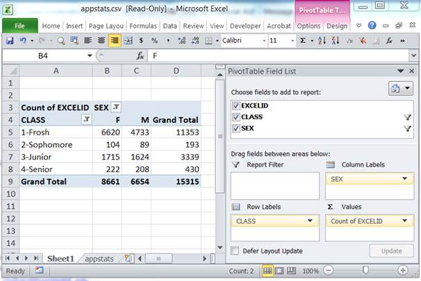
To generate report using your data, you will probably want to use an Excel pivot table. Although there are many options available, here is a very quick summary to produce a simple table. Assume you have a table showing people who have received degrees with the following columns: Name, Term, Degree, and Sex.. The goal of this pivot table is to count the number of students by sex who received different degrees.

Start by choosing Data; Pivot Table and Pivot Chart report. (In Excel 2007, Pivot tables are on the Insert/Tables menu.) Click Next to select a pivot table from the current spreadsheet; click Next to accept the default range of data; click Finish to create a blank pivot table in a new worksheet. You will now see a blank table and a list of your column names. To create this example, drag the Degree field name to the Row Fields, Sex to the Column Fields, Term to the Page Fields, and Name to the Data Items. You will now see Sex by Degree counts and totals for all terms in the data. To view a particular term, you can use the drop-down on the Term field at the top and the counts will instantly adjust to show counts for the term selected. The result may look something like:

term	Fall
Count of name	sex
degree	F	M	Grand Total
BS	9	6	15
MS	1	4	5
Grand Total	10	10	20

You may also drag more than one field to the row, column, or page fields to create much more complex reports. A great deal more information about creating Pivot Tables is available through the Help in Excel.